This is an overview of the work done on this project. Detailed report is here.

Introduction

In RDF Graphs Analyzer we furthered an existing project which enables the users to traverse large RDF graphs. Our research in the project included implmentation of some important measures inside the graph by preprocessing the data and enabling the users to give a starting point. The project is available as open source here. The front end for graph traversal looks like the following.

The graph enables its users to click on different nodes. You can traverse the graph while also analyzing important information of the graph. Since these are huge graphs with a lot of nodes. A lot of people are unable to decide where they should start their graph traversal from. For this, we implemented two methods which gives you an initial number of important starting nodes calculated based on different important measures including how connected these nodes are i.e node centralities and node rankings which are the importance of those nodes based on how other nodes are pointing to it.

Page Rank

For implementing node rankings, we took the approach of implementing the initial starting nodes of the graph using page rank algorithm. Starting from an initial ranking of the nodes based on the number outdegrees of each node. The algorithm keeps running in a loop until it converges to the final ranks for each node. This is done by first calculating an adjacency matrix of the graph and than moving on to calculate the rankings of each nodes based on the number of nodes pointing to it after the first step. You can read more about pagerank here and here.

As seen in the above figure. The page rank applied to the DAQL dataset gives us the following results. Where the number in brackets for reach node represents their rank for that graph. The code for the algorithm was implemented using Apache Spark Java and is available as open source here.

Centralities

There was an alternative way through which we went about calculating the starting nodes for our users. This method through which we calculate the nodes importance based on their connectedness is called node centrality. There are three types of centralities you can calculate for a node.

• Degree Centrality
• Closeness Centrality
• Betweenness Centrality

We only focused on calculating the first two centralities for all the nodes of the graphs.

Degree Centrality

Degree centrality is simply the measure of number of out degrees and in degrees of a graph. We calculated this for each node on the fly while the user is using the software.

Closeness Centrality

The closeness centrality for a graph required us to calculate the shortest paths for each node to all the other nodes. This gave rise to the problem of using the shortest path algorithm.

Hence in order to calculate the closeness centrality we first went about implementing a single source shortest path algorithm for a node in a graph. Since we were dealing with non-weighted directed graph. We used BFS algorithm with the MapReduce technique to calculate the shortest path for a node. The implementation of the algorithm can be found here.

The next step was to find the nodes which will be most central in the graph. For this we took the advantage of the basic definition of closeness centrality which define a centrality for the node as the inverse sum of the shortest path of that node with all the other nodes. This helped us realize that if we continously and parallely hop back from the top 10% nodes with maximum out-degrees to the farthest nodes in the graph ignoring cycles and loops. We can find out the nodes in the graph which are the intersections. By intersection we mean, the nodes which are connected to the maximum nodes in those 10% nodes we selected at the start. If we found the nodes with maximum intersections, we'll find the nodes which are connected to the maximum number of nodes. Let's take an example of it. To understand the example. We start with the help of a figure.

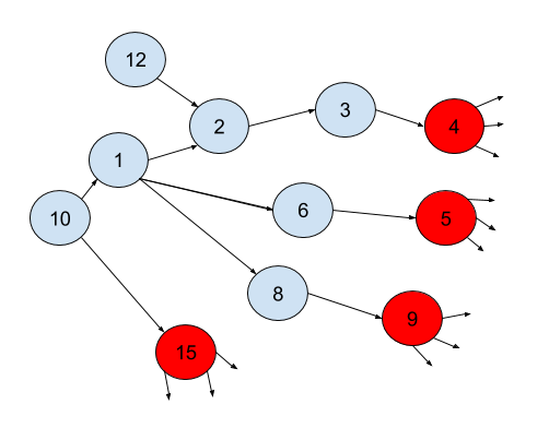
In the above figure we consider the red nodes as the 10% nodes with max out-degrees. Now if we keep going by hop by hop paralelly from each red node we'll come up with a tabular data that will give us the distances of each red node from all the other nodes. For example, the distance of node 9 to node 1 is 2. While the distance of node 4 to node 10 is 4.

This will give us a final result like this.

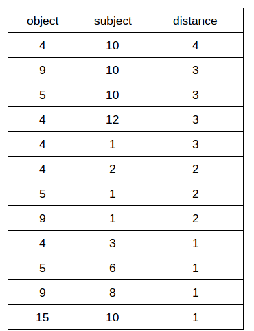
Where object are the red nodes while subject are the rest of the nodes. Once we found this out, we can simply group our data with respect to the subjects in order to find the maximum count of intersections for that subject. In the above example, node 10 will be the one connected to the maximum number of nodes which will result in it having a higher closeness centrality. The algorithm for finding the closeness nodes can be found here.

Once we found these maximum intersection nodes. We feed them to the BFs algorithm defined above which gives us the shortest path of those nodes to all the other nodes. Than we pass the sum of our shortest path distances of those nodes to the closeness centrality formula to give us our final closeness centralities.

Our final results with highest page rank nodes at the left and highest closeness centrality nodes at the right looks like this.

Note: The project was implemented in University of Freiburg as part of a Master project within the University with other team members.